VisionRT
Deterministic Inference via Vertical Optimization — blog
VisionRT is a case study in vertical optimization. How do you take a computer vision pipeline and reduce overhead so drastically that you can predict to the microsecond when it will finish?
This matters because safety-critical real-time systems don't just need fast inference, they need predictable inference. A pipeline that averages 10ms but occasionally spikes to 30ms can miss deadlines and drop frames.
The philosophy here is creating a system sculpted for our specific use case by optimizing every layer from frame capture to model execution.
The end result is a pipeline that processes frames so efficiently it just waits for the camera:
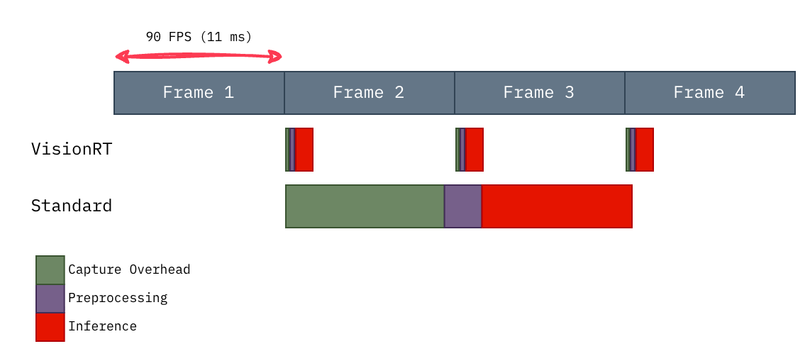
Fig. 1: VisionRT fits within the 90 FPS frame budget. The baseline pipeline struggles to keep up.
Here's how we got there.
1. Finding the Bottleneck
Throughout the rest of the blog, I will use nsys to profile the image classification pipeline in search of potential areas for optimization.
The pipeline is split into 3 stages:
- Capture - Fetching the frame buffer.
- Preprocessing - Creating a PyTorch-compatible tensor.
- Inference - ResNet50's forward propagation.
These stages are abstracted in the following profiled code:
@nvtx.annotate("standard", color="blue")
def run_standard(cap, model):
    frame = capture_overhead(cap)
    if frame is False:
        return False

    tensor = preprocessing(frame)
    inference(tensor, model)

    return True
Here are the summary after profiling 10K samples post-warmup:
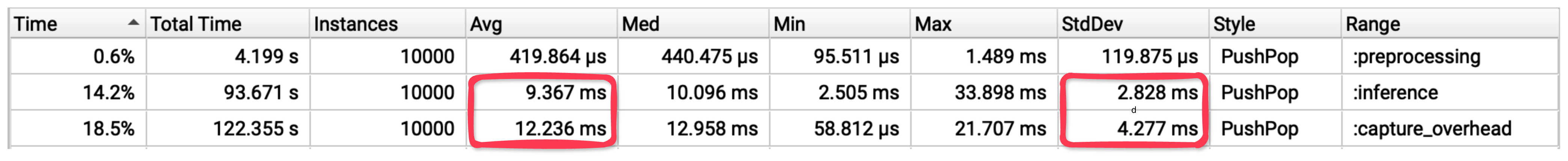
Fig. 2: Result of profiling with nsys and nvtx
Capture and Inference dominate the latency with an average of 12.2 ms and 9.4 ms, respectively. We also observe significant variance in both stages' latency, which can violate real-time system requirements.
Assuming average latency, let's analyze the potential cascading effect.
2. Quantifying the Impact
For our baseline pipeline with negligible preprocessing overhead:
- Mean capture latency:
12.2 ms - Mean inference latency:
9.4 ms - Total pipeline latency:
21.6 ms per frame
The camera operates at 90 Hz, establishing a frame period of 11.11 ms. This represents our real-time budget, the maximum processing time to maintain synchronous operation.
With 21.6 ms actual processing time, we accumulate 10.49 ms of delay per frame processed. This deficit compounds deterministically:
Analysis over 100 frames:
| Measurement | Calculation | Time |
|---|---|---|
| Processing time | 100 * 21.6 ms |
2,160 ms |
| Real time elapsed | 100 * 11.11 ms |
1,111 ms |
| Accumulated deficit | 2,160 ms - 1,111 ms |
1,049 ms |
This 1.05 second deficit corresponds to 94 dropped frames (1,049 ms // 11.11 ms), over the course of processing 100 frames.
| Metric | Calculation | Result |
|---|---|---|
| Efficiency | 100 frames processed / 194 frames produced |
51.4% |
| Effective throughput | 51.4% * 90 FPS |
46.3 FPS |
The baseline pipeline is therefore latency-bound by a factor of ~2x, explaining the observed degradation from 90 FPS to ~45 FPS under sustained load. The system cannot operate at the camera's native frame rate.
Now we'll determine whether to target Capture or Inference first. To maximize potential gains, we'll calculate their lower bound to see which stage has more headroom.
3. Calculating the Lower Bound
Pipeline Specifications:
| Component | Specification | Value |
|---|---|---|
| Resolution | 320 x 240 | 76,800 pixels |
| Frame Format | YUYV (4:2:2) | 2 bytes/pixel |
| Frame Buffer | 320 x 240 x 2 | 153.6 KB |
| Refresh Rate | 90 Hz | 11.11ms period |
| Interface | USB 2.0 | 60 MB/s bandwidth |
| GPU PCIe | RTX 5080 | 960 GB/s bandwidth |
| GPU FPU | RTX 5080 | 56.28 TFLOPS |
3.1 Capture Lower Bound
To establish a theoretical minimum for capture, I'll trace the data flow from camera to GPU-ready tensor.
Technical details (optional)
3.1.1 Frame Acquisition Time
| Operation | Calculation | Time |
|---|---|---|
| Camera frame period | 1 / 90 Hz |
11.11ms |
| USB 2.0 transfer | 153.6 KB / 60 MB/s |
2.02ms |
| Frame acquisition | max(11.11ms, 2.02ms) |
11.11ms |
3.1.2 Preprocessing Kernel Time
| Operation | Calculation | Result |
|---|---|---|
| Threads | 153.6 KB / 4B |
38.4K threads |
| Integer unpacking | 56 ops x 38.4K threads |
Not limiting |
| Compute | (12 ops x 38.4K threads) / 56.28 TFLOPS |
8.2ns |
| Memory | (28 bytes x 38.4K threads) / 960 GB/s |
1.12us |
| Kernel time | max(compute, memory) |
1.12us |
Altogether, the capture stage yields a lower bound of approximately 11.11ms. The overwhelming majority of the latency comes from acquiring the frame itself.
3.2 Inference Lower Bound
To establish a theoretical minimum for inference, I'll analyze the computational requirements of ResNet50 by examining a single convolution operation and scaling to the full network.
Down the rabbit hole: Conv2d kernel analysis
3.2.1 Analyzing Conv2d Operations
I wrote a naive 2D convolution kernel to understand the exact operations required:
    // block parallelize over the first three for-loops.
    const int batch = blockIdx.x * blockDim.x + threadIdx.x;
    const int out_channel = blockIdx.y * blockDim.y + threadIdx.y;
    const int out_row = blockIdx.z * blockDim.z + threadIdx.z;

    if (batch >= bs || out_channel >= out_ch || out_row >= out_h) {
        return;
    }

    // thread parallelize over the the 4th for-loop.
    for (int out_col = threadIdx.x; out_col < out_w; out_col += blockDim.x) {

      auto dot_product = (T) 0;

      for (int in_channel = 0; in_channel < in_ch; in_channel += 1){
            for (int filter_row = 0; filter_row < f_h; filter_row += 1){
                for (int filter_col = 0; filter_col < f_w; filter_col += 1){

                    const T filter_element = filter[out_channel][in_channel][filter_row][filter_col];

                    const int image_row = filter_row + out_row * stride;
                    const int image_col = filter_col + out_col * stride;
                    const T image_element = image[batch][in_channel][image_row][image_col];

                    dot_product += filter_element * image_element;
                }
            }
        }

        out[batch][out_channel][out_row][out_col] = dot_product;
    }
Each output element requires approximately:
| Metric | Formula |
|---|---|
| Compute | ceil(out_w / blockdim.x) x (in_ch x f_h x f_w) MACs |
| Memory | 4 x ceil(out_w / blockdim.x) x [2 x (in_ch x f_h x f_w) + 1] Bytes |
Note: out_w = 1 + (in_h - f_h) // stride
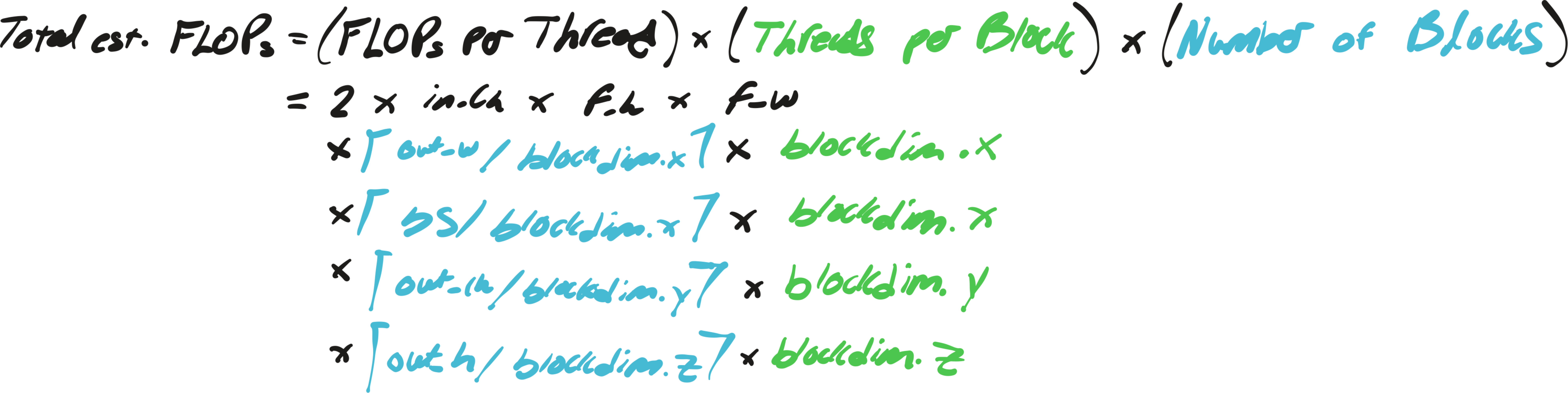
The formula for the kernel's total FLOPs and MBs, assuming all threads launched do work, become the following:
| Metric | Formula |
|---|---|
| FLOPs per Thread | 2 x ceil(out_w / blockdim.x) x in_ch x f_h x f_w |
| MBs per Thread | 4 x ceil(out_w / blockdim.x) x [2 x (in_ch x f_h x f_w) + 1] x 1e-6 |
| Threads per Block | blockdim.x x blockdim.y x blockdim.z |
| Number of Blocks | ceil(bs / blockdim.x) x ceil(out_ch / blockdim.y) x ceil(out_h / blockdim.z) |
| Total est. FLOPs | FLOPs per Thread x Threads per Block x Number of Blocks |
| Total est. MBs | MBs per Thread x Threads per Block x Number of Blocks |
Note: Each multiply-accumulate (MAC) counts as 2 FLOPs
Despite the verbosity, the total FLOPs can be nicely simplified into the following well-known formula when the tensor shapes are "nice".
Total FLOPs = 2 x bs x (f_h x f_w x in_ch) x (out_h x out_w x out_ch)Note: Total FLOPs <= Total est. FLOPs - shown in Appendix I
3.2.2 Compute or Memory Bound?
We'll use a simple example to determine whether this kernel is compute or memory bound, assuming the following launch config:
dim3 threadGrid(8, 8, 4); // 256 threads per block
dim3 blockGrid(
    (bs + 7) / 8, // batch dimension
    (out_ch + 7) / 8, // out channel dimension
    (out_h + 3) / 4 // out height dimension
);
Given a 226x226 RGB image, 3x3 filter, and parameters [stride=1, out_ch=64]:
| Per-Thread | Calculation | Result |
|---|---|---|
| out_w iters | ceil(224 / 8) |
28 iterations |
| MACs | 28 x (3 x 3 x 3) |
756 MACs |
| reads | 756 x 2 elements x 4B |
6,048 bytes |
| writes | 28 elements x 4B |
112 bytes |
| FLOPs | 756 x 2 |
1,512 FLOPs |
| Total memory | 6,048 + 112 |
6,160 bytes |
| Device-Wide | Calculation | Result |
|---|---|---|
| Total Threads | 1 batch x 8 out_ch_blocks x 56 out_h_blocks x 256 threads/block |
114,688 threads |
| Compute | (1,512 ops x 114,688 threads) / 56.28 TFLOPS |
3.08 us |
| Memory | (6,160 bytes x 114,688 threads) / 960 GB/s |
0.736 ms |
| naive Kernel time | max(compute, memory) |
0.736 ms |
The kernel is clearly memory-bound. Based on this analysis, we'd expect convolution to take around 0.7 ms.
However, when profiling convolution directly on PyTorch
@nvtx.annotate("conv_pytorch", color="black")
def conv(x, w):
    return F.conv2d(x, w, stride=[1,1])
the results were shocking:

Fig. 3: Result of profiling cuDNN convolution
The convolution kernel averaged just 15 us and a minimum of 14.8 us! Surprisingly, this actually aligns with the following formula for the optimal kernel, where data is moved only once for input, weight, and output.
| Calculation | Result | |
|---|---|---|
| Input | 4 x bs x in_ch x in_h x in_w |
612912 bytes |
| Weight | 4 x f_h x f_w x in_ch x out_ch |
6912 bytes |
| Output | 4 x bs x out_ch x out_h x out_w |
12845056 bytes |
| cuDNN Kernel time | (Input + Weight + Output) / 960 GB/s |
0.14 us |
Knowing this we can extrapolate the same formula to the entire model to find the lower bound, with the assumption that memory bandwidth is the limiting factor.
Below is the ResNet50 architecture, the core convolution operations are boxed in light red:
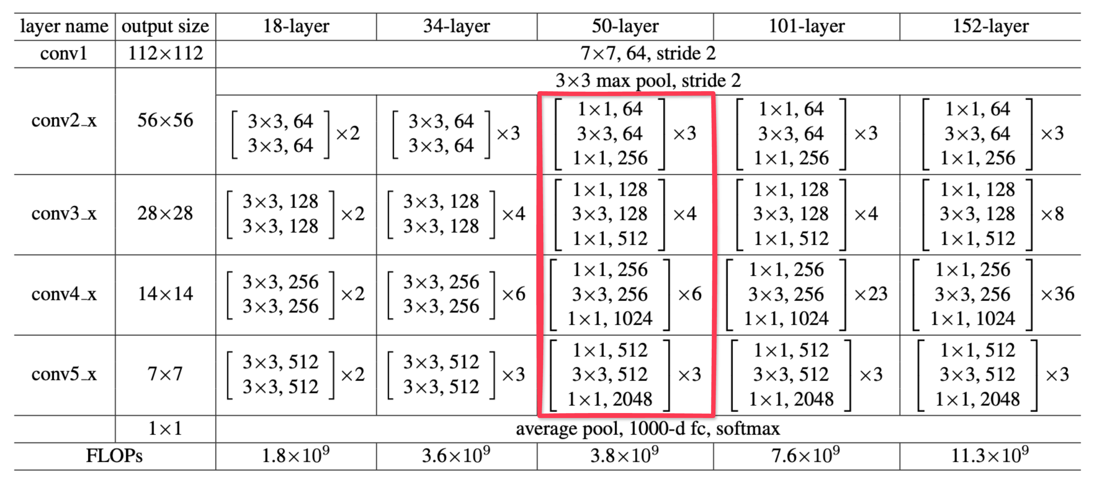
Fig. 4: ResNet model architecture, taken from "Deep Residual Learning for Image Recognition" by Kaiming He et al. (2015).
| Stage | Calculation | Latency |
|---|---|---|
| conv1 | 7.67 MB / 960 GB/s |
0.01 ms |
| conv2 | 31.36 MB / 960 GB/s |
0.03 ms |
| conv3 | 30.54 MB / 960 GB/s |
0.03 ms |
| conv4 | 45.97 MB / 960 GB/s |
0.05 ms |
| conv5 | 64.99 MB / 960 GB/s |
0.07 ms |
| fc | 8.2 MB / 960 GB/s |
0.01 ms |
| Inference lower bound | conv1 + ... + conv5 + fc |
0.2 ms |
So inference yields a lower bound of approximately 0.2ms, which does seem a bit too low. In fact, I might even be off here, but the exact number isn't what matters. What's clear is that inference has plenty of overhead to minimize.
Here are the lower bounds compared side by side:
| Stage | Lower Bound | Headroom | Possible Reduction in Latency (%) |
|---|---|---|---|
| Capture | 11.11ms | 1.126ms | 9% |
| Inference | 0.2ms | 9.167ms | 98% |
So knowing that Inference has significantly more headroom than Capture, let's take a closer look into Inference...
4. Optimizing Inference
During inference, two main time sinks stand out: the overhead of scheduling computations, and the computations themselves. Here, we'll focus on optimizing both by leveraging CUDA graphs and the PyTorch compiler.
Skip or dive deep
4.1 Eliminating Scheduling Overhead
@nvtx.annotate("inference", color="red")
def inference(tensor, model):
    _ = model(tensor)
    torch.cuda.synchronize()
Here we zoom into a single Inference sample on the profiler:
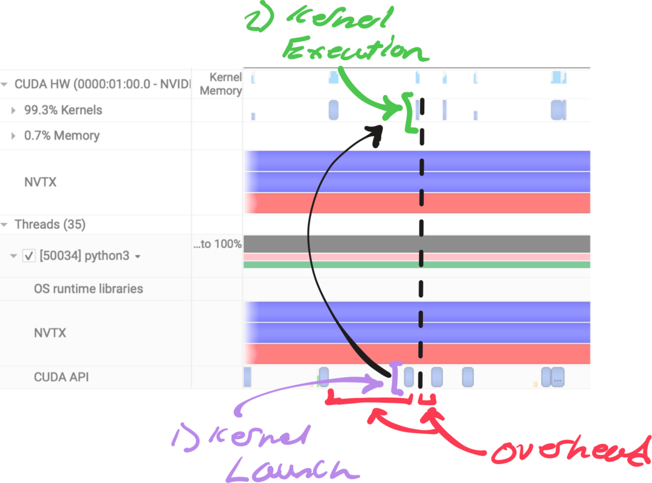
Fig. 5: An annotated view of ResNet50 inference on nsys's profiler
Fig. 5 is how the profiler looks for every GPU kernel executed. For each kernel the following work must be done.
- CPU work - Framework overhead and CPU computation before launch.
- Kernel Launch - CPU enqueues kernel into CUDA stream.
- GPU Scheduling - GPU schedules kernel when resources are met.
- Kernel Execution - GPU performs computation asynchronously.
- Synchronization (if needed) - Host blocks on CUDA sync or blocking API call.
We can minimize the overhead and jitter surrounding kernel execution by capturing the CUDA graph and replaying it each iteration with a single kernel launch as long as the shapes and computation remain static.
Here we record the computational graph of the forward function fn from PyTorch's default CUDA stream.
cudaStreamBeginCapture(stream, cudaStreamCaptureModeGlobal);
{
    c10::cuda::CUDAStream capture_stream = c10::cuda::getStreamFromExternal(stream, 0);
    c10::cuda::CUDAStreamGuard guard(capture_stream);

    out.copy_(fn(in).cast<torch::Tensor>());
}
cudaStreamEndCapture(stream, &graph);
Ideally, this will eliminate the white space between each Kernel Execution in Fig. 5. The diagram below illustrates this conceptually, notice how the idle periods and delays (crossed out in pink) are removed when using CUDA graphs:
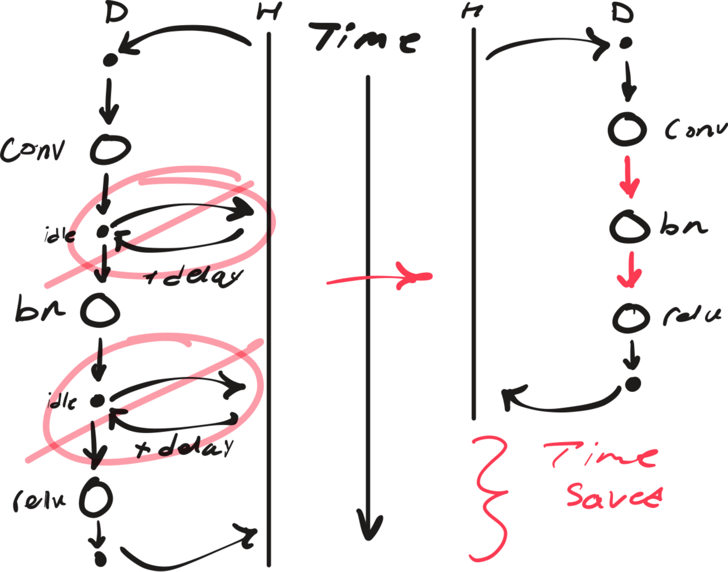
Fig. 6: Conceptual illustration to show the benefit of CUDA graphs.
The black arrows represent the overhead/latency of CPU(H)-GPU(D) coordination.
To see this overhead in the profiler, we can zoom into the CUDA API calls before and after each convolution kernel:
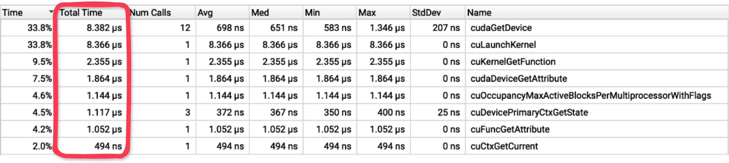
Fig. 7: nsys view focused on CUDA API calls around kernel execution.
Note: Profiled with --cuda-trace-all-apis=true
Nearly 28 microseconds of CUDA API calls occur before and after the kernel executes!
Overall, Fig. 6 demonstrates how graph capture and replay eliminates communication between each operation, significantly reducing end-to-end latency. For workloads with many small kernels, this overhead can dominate execution time.
4.2 Accelerating Computation
While CUDA graphs eliminates scheduling overhead, we can focus on reducing the time on device by optimizing what happens within the graph.
PyTorch's torch.compile is a simple to use tool that generates highly efficient Triton kernels. Underneath this tool exists a sophisticated native JIT compiler infrastructure:
- TorchDynamo - Captures Python code into a computational graph.
- Torch.fx - Intermediate representation that makes graph transformation easy.
- TorchInductor - Generates optimized Triton kernels from the graph.
Let's see what inductor generates by default.
compiled_model = torch.compile(model, backend="inductor", dynamic=False)Inspecting the generated code reveals the following kernels:
triton_poi_fused__native_batch_norm_legit_no_training_relu
triton_poi_fused__native_batch_norm_legit_no_training_add_relu
extern_kernels.convolution
inductor already fused the batch norm with ReLU, and occasionally the residual add, but left convolution to an external kernel, typically implementations in cuDNN or CUTLASS, which are hard to beat.
This is great. However, we don't actually need to compute batch normalization at inference time at all. In fact, constant folding the normalization into the convolution parameters is a common optimization pattern, eliminating an entire kernel and memory round-trip.
Let's create the FX graph transformation:
if node.op == "call_function" and node.target == F.batch_norm:
    if parent.op == "call_function" and parent.target == F.conv2d:
        ...
        inv_sqrt_var_eps = (var.value + eps) ** -0.5
        convW_new = convW.value * (bnW.value * inv_sqrt_var_eps).view(-1, 1, 1, 1)

        if not convBias: create_bias(parent)
        convBias_new = (convBias - mean.value) * bnW.value * inv_sqrt_var_eps + bnBias.value
Note: The derivation for the folded parameters is found in Appendix II.
And now the custom backend:
@register_backend
def visionrt(gm: fx.GraphModule, ins):
    if config.custom_optims:
        ...
        gm, ins = optimize_fx(
            gm=gm,
            placeholders=placeholders,
            transformations=[xform for _, xform in enabled_xforms]
        )
    return compile_fx(gm, ins) # pass to inductor
We now observe that inductor generates a few different kernels:
triton_poi_fused_convolution_relu
triton_poi_fused_add_convolution_relu
extern_kernels.convolution
Matching a similar pattern as before, inductor is fusing convolution with ReLU, and the residual add if present. The following is a visual on how the computation graph was optimized:
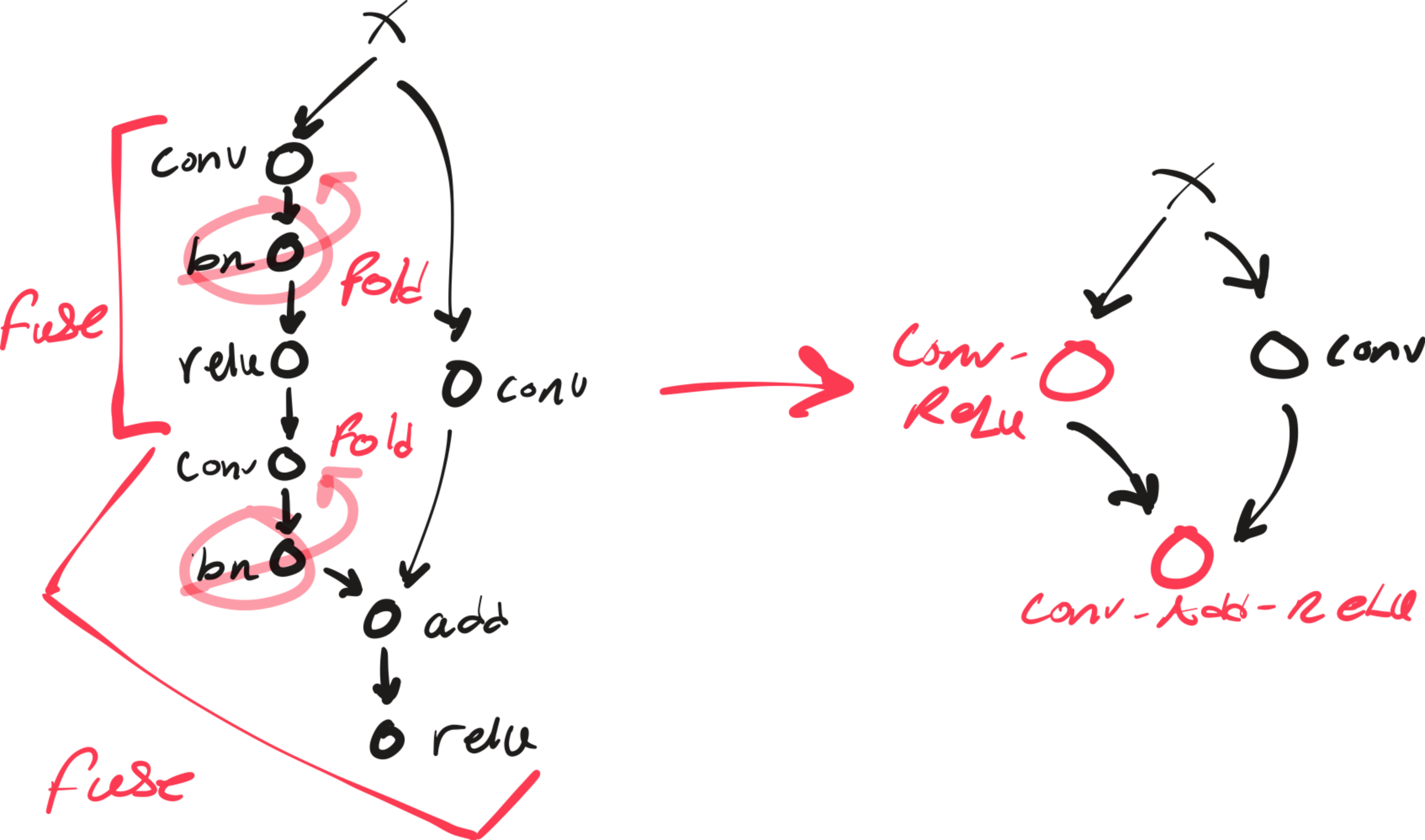
Fig. 8: Before and after graph transformations
We can see how conv-bn folding created opportunities for inductor to fuse other operations with convolution by eliminating the batch norm barrier.
While I was inspecting the generated Triton code for the conv_relu and add_conv_relu kernels:
x2 = xindex
x0 = (xindex % 256) # folded bias index
tmp0 = tl.load(in_out_ptr0 + (x2), xmask)
tmp1 = tl.load(in_ptr0 + (x0), xmask, eviction_policy='evict_last')
tmp2 = tmp0 + tmp1 # bias add
tmp3 = tl.full([1], 0, tl.int32)
tmp4 = triton_helpers.maximum(tmp3, tmp2)
tl.store(in_out_ptr0 + (x2), tmp4, xmask)
I noticed that the new bias appeared, confirming that our transformation worked!
I also implemented manual fusing transformations such as conv_relu, add_relu, and add_conv_relu using CUDA, Triton, and cuDNN. However, they all resulted in regressions or negligible improvements that ruined the model's flexibility.
Working with inductor was clearly the better approach.
The figure below highlights the significant drop in inference times achieved with these optimizations:
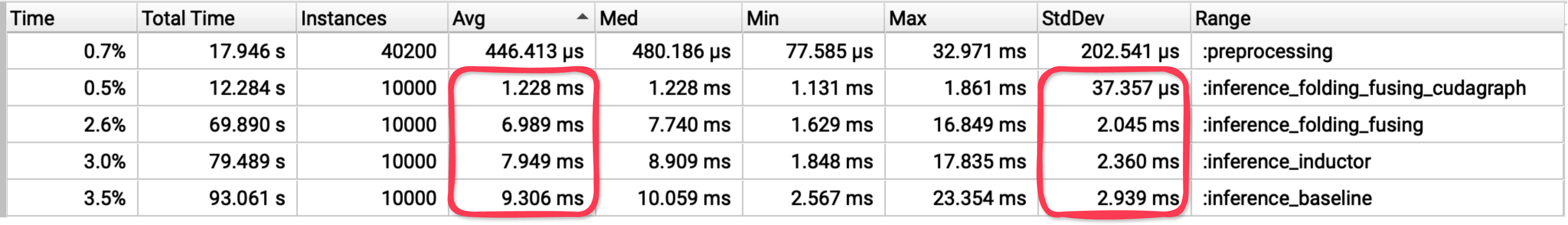
Fig. 9: Result of profiling post inference optimizations with nsys and nvtx
These results are broken down to reveal the incremental improvements in both latency and predictability from each optimization:
| Version | Avg Latency | Latency Reduction | StdDev | Variance Reduction |
|---|---|---|---|---|
| Baseline | 9.306 ms | - | 2.939 ms | - |
| Inductor | 7.949 ms | 14.6% | 2.360 ms | 19.7% |
| Folding + Inductor (Fusing) | 6.989 ms | 24.9% | 2.045 ms | 30.4% |
| Folding + Inductor (Fusing) + CUDA Graph | 1.228 ms | 86.8% | 37.357 us | 98.7% |
Note: Profiling script found here
The average inference latency drops from 9.3ms to just 1.2ms (86.8% reduction), and the standard deviation has decreased dramatically from 2.9ms to just 37us!
Inference times are so predictable, it's practically deterministic. Notice how the median equals the average, implying a nearly perfect normal distribution.
Now that Inference is no longer a bottleneck, let's tackle Capture overhead.
5. Optimizing Capture
Let's revisit the profile summary used to determine the bottlenecks shown in Fig. 2.
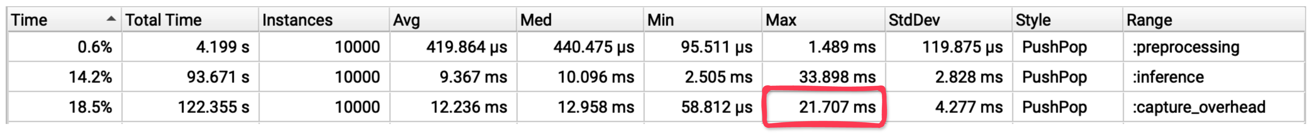
Fig. 10: Result of profiling the baseline with nsys and nvtx
Recall that we calculated the headroom for optimization to be only around ~1ms, so we'll mostly focus on writing a fast path with zero unnecessary overhead, as we are not bound by the design decisions large general frameworks like OpenCV are.
As discussed in our lower bound calculation, this section will focus on creating a pipeline that requires only a single memcpy and a minimal preprocessing kernel.
Implementation details inside
5.1 Streaming Frames
To interface with any hardware, we need drivers. V4L2 (Video4Linux2) is a low-level Linux API that provides a collection of device drivers for real-time video capture.
To guide development, I designed the camera module to be conveniently used from Python as follows:
camera = Camera("/dev/video0")
for frame in camera.stream():
    ....
So we'll need to implement a streaming function, along with low-level systems programming tasks such as managing file descriptors, checking camera compatibility, selecting a format, and providing other convenience functions.
5.1.1 The Boring
// File descriptor management
int open_camera(const char*);
void close_camera(void);

// Camera compatibility check
void validate_capabilities(void);

// Format selection
void discover_formats(void);
void set_format(size_t);

// Convenience methods
void list_formats(void);
void print_format(void);
5.1.2 The Not-So-Boring
Best Camera Format?
Aside from streaming, the only other feature beyond the boring ioctl calls was automatically selecting the best format for convenience. To the user, the only attributes of a camera format that matter is its resolution and framerate, which are inversely correlated due to the camera's fixed bandwidth. For example, a higher resolution requires more bandwidth, thus more time, resulting in a lower framerate. So if we want a higher framerate, we need to select a lower resolution. I experimented with a heuristic that seems to work well enough:
\[ \text{score} = \alpha \cdot \log\left( \sqrt{\text{width} \cdot \text{height}} \right) + \beta \cdot \log(\text{fps}), \]It's pretty straightforward. The score combines the framerate with a "linearized" resolution, achieved by taking the square root of the product of width and height. Applying the logarithm helps with "numerical stability", while the alpha and beta weights determine the relative importance of each factor.
Streaming:
We'll first need a ring buffer, V4L2 will manage the scheduling for the ring buffer under the hood, I just need to provide the buffers where the dequeued frame will be stored in. Also, V4L2 allows for mmap-streaming if the camera is compatible. Meaning we can avoid an entire memory copy by memory mapping the frame buffers directly from kernel space into user space!
// Psuedo ring buffer
class CameraRingBuffer{
    struct CameraBuffer {
        void* start;
        v4l2_buffer v4l_buf;
    };

    CameraBuffer* buffers;
    ...
}

// Memory mapping
buffer.start = mmap(NULL, buffer.length(), PROT_READ | PROT_WRITE, MAP_SHARED, fd, buffer.v4l_buf.m.offset);
We also need to wrap the data in the buffer into a usable tensor on the device:
torch::Tensor get_frame(size_t idx) {
    void* src = h_ring.buffer_start(idx);
    size_t size = h_ring.buffer_length(idx);

    auto options = torch::TensorOptions()
        .dtype(torch::kUInt8)
        .device(torch::kCUDA);

    auto frame = torch::empty(..., options);

    cudaMemcpy(frame.data_ptr(), src, size, cudaMemcpyHostToDevice);

    return frame;
}
Finally, to complete the API design aforementioned, we need to create a Pythonic iterable that yields a frame as soon as a buffer is dequeued:
torch::Tensor __next__() {
    if (!cam->is_streaming) {
        cam->start_streaming();
    }

    int idx = cam->dequeue_buffer();
    if (idx == -1) {
        throw py::stop_iteration();
    }

    auto frame = cam->get_frame(idx);
    cam->queue_buffer(idx);

    return frame;
}
The Camera module is now complete, and the frame acquisition process is depicted as follows:
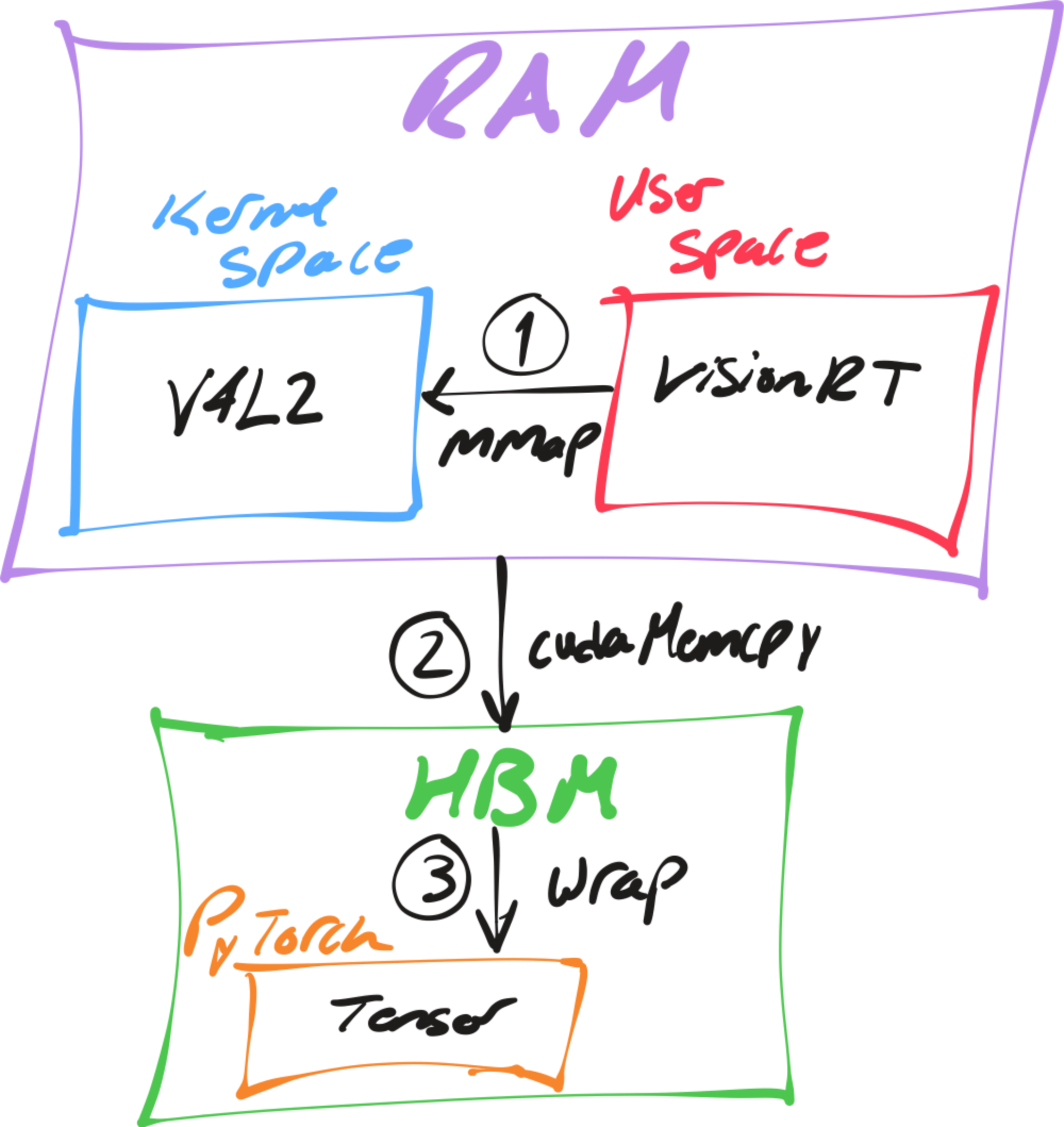
Fig. 11: Schematic of the VisionRT camera frame acquisition pipeline.
You may have noticed there's no decoder in this pipeline. Thats because I intentionally avoided compressed pixel formats to eliminate the need for a decode step, thus removing its potential latency overhead entirely. But there is a tradeoff, we are limited to uncompressed, lower-resolution feeds, but this is reasonable for most computer vision models.
However, now the frames are in a colorspace (YUYV) that is not compatible with most modern pretrained computer vision models, so we need to preprocess them.
5.2 Preprocessing Frames
I made sure to decouple preprocessing from frame acquisition, allowing users to apply their own preprocessing functions at the Python level, as follows:
def preprocess(x: torch.Tensor):
    ...

camera = Camera("/dev/video0")
for frame in camera.stream():
    frame = preprocess(frame)
    ...
ResNet expects input tensors in normalized RGB color format, arranged as (batch_size, channels, height, width). The YUYV format from the camera encodes color differently, each pixel pair shares UV (chroma) values to save bandwidth.
The naive approach using standard libraries:
rgb = cv2.cvtColor(frame, cv2.COLOR_YUYV2RGB) # colorspace conversion
chw = np.transpose(rgb, (2, 0, 1)) # reshaping
tensor = torch.from_numpy(chw).unsqueeze(0).cuda().float() # memory copy
tensor = ((tensor / 255.0) - mean) / std # normalization
This process results in multiple memory roundtrips for each frame.
However, by using a custom preprocessing kernel that fuses colorspace conversion, normalization, and reshaping into a single operation, we can reduce these memory roundtrips to just one.
CUDA
__global__ void yuyv2rgb_kernel(
    const uint32_t* yuyv,
    float* rgb,
    int num_pairs,
    int stride,
    float scale_r, float scale_g, float scale_b,
    float offset_r, float offset_g, float offset_b
)
Triton
@triton.jit
def _yuyv2rgb_kernel(
    yuyv_ptr,
    out_ptr,
    stride,
    num_pairs,
    SCALE_R: tl.constexpr, SCALE_G: tl.constexpr, SCALE_B: tl.constexpr,
    OFFSET_R: tl.constexpr, OFFSET_G: tl.constexpr, OFFSET_B: tl.constexpr,
    BLOCK_SIZE: tl.constexpr,
) -> None
You can view the full implementations here:
- CUDA: csrc/kernels.cu
- Triton: visionrt/preprocess.py
5.3 Was it Worth It?
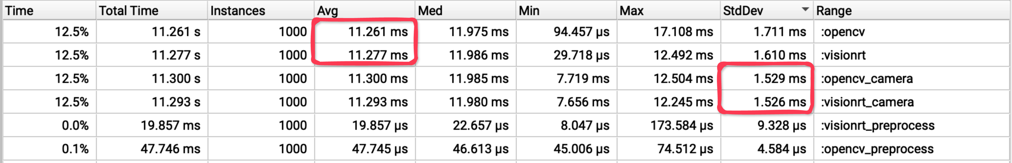
Fig. 12: Result of profiling capture and preprocessing
Well, no-not really, we only shaved off like 20 us from preprocessing.
Honestly, that was expected. However, our efforts were not entirely wasted. We observed that both cameras exhibit a high standard deviation of over 1.5 ms. Now that we have full control over the camera, we can pace frame capture to ensure frames are received exactly at the expected frame interval.
Looking more closely at Fig. 11, we see that the frame period fluctuates between the expected 11.3 ms and an unexpected 7.7 ms, meaning standard deviation is caused by the frames dequeuing too early.
So addressing the jitter is simple, I will introduce a mechanism to wait for the remainder of the frame interval by sleeping as needed:
if (deterministic_ && last_frame_time_) {
  Duration target_interval(1.0 / fps());
  auto elapsed = Clock::now() - *last_frame_time_;
  if (elapsed < target_interval) {
    std::this_thread::sleep_for(target_interval - elapsed);
  }
}
Now we should expect a the significant drop in standard deviation since we have implemented pacing:
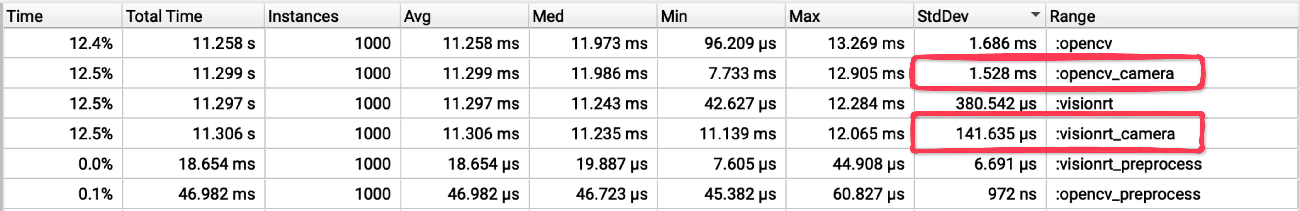
Fig. 13: Result of profiling capture and preprocessing after pacing
These results are broken down below to highlight the improvements for capture:
| Version | Avg Latency | Latency Reduction | StdDev | Variance Reduction |
|---|---|---|---|---|
| Baseline | 11.3 ms | - | 1.53 ms | - |
| V4L2 | 11.3 ms | 0% | 1.53 ms | 0% |
| V4L2 + Pacing | 11.3 ms | 0% | 141.635 us | 99.1% |
Note: Preprocessing was negligible and thus omitted from the table.
With just pacing we have reduced the standard deviation from 1.529 ms to just 141.635 us!
6. Surprisingly Deterministic

Fig. 15: Result of profiling visionrt and the baseline end-to-end.
| Version | Avg Latency | Latency Reduction | Overhead | Overhead Reduction | StdDev | Variance Reduction |
|---|---|---|---|---|---|---|
| Baseline | 21.8 ms | - | 10.7 ms | - | 5 ms | - |
| VisionRT | 11.3 ms | 48.2% | 0.2 ms | 98.1% | 137 us | 99.9% |
200 us with a jitter of 137 us, predominantly coming from capture. We have reduced the overhead by so much that the average latency is now practically limited only by the camera's refresh rate!
Here is a nice histogram on the profiling trace:
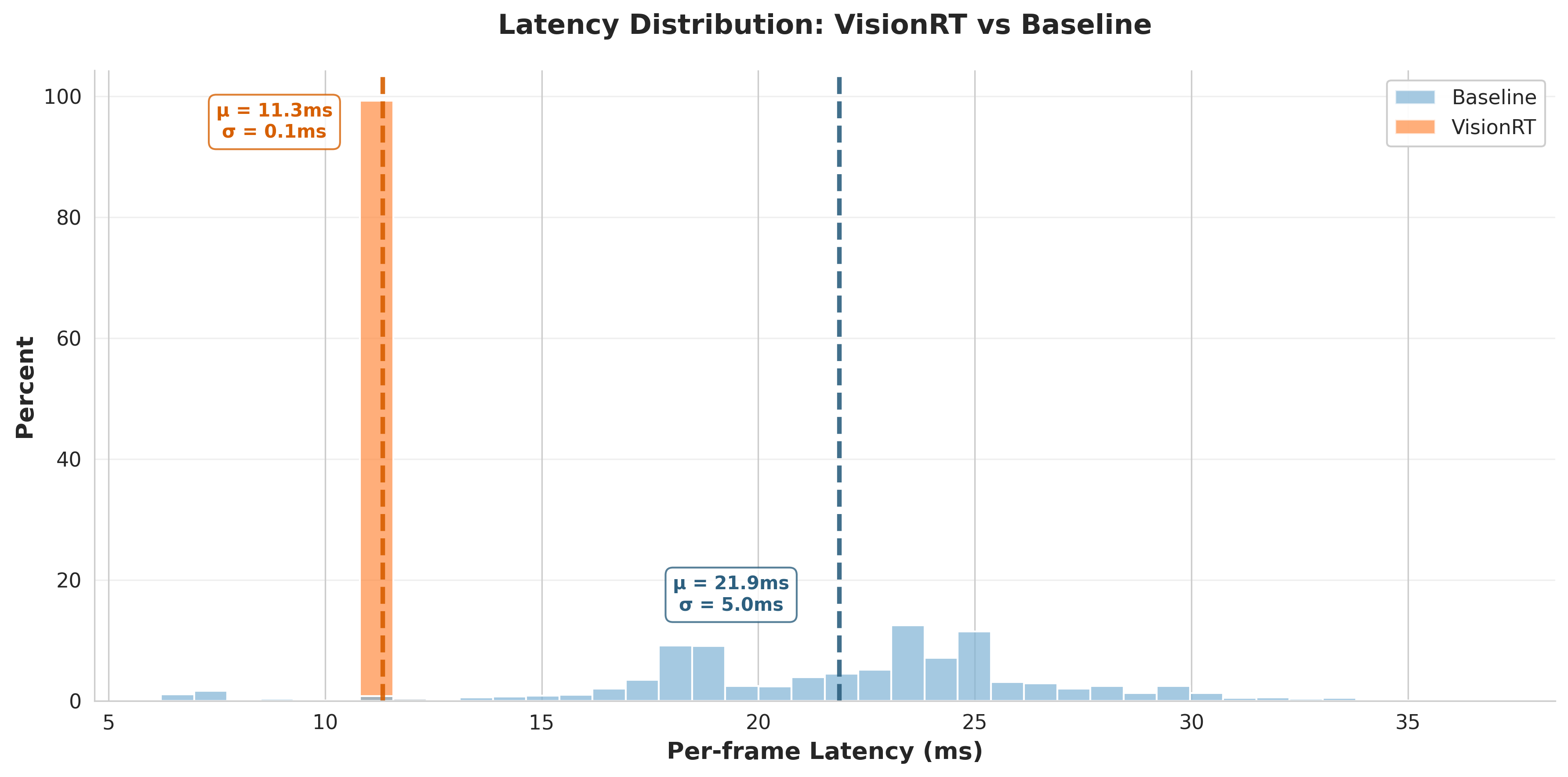
Fig. 16: visionrt achieves deterministic sub-12ms latency while the baseline varies unpredictably from 20-30ms
This orange narrow peak shows that we can expect image classifcation to complete at the webcam's refresh rate nearly 100% of the time. In other words, visionrt is so fast and deterministic that are practically measuring the hardware!
7. Appendix
Contains extra technical details referenced in the main text.
Expand for appendix (optional)
7.1 Appendix I
Showing that Total est. FLOPS is the upper bound for Total FLOPs.
Step 1. Expand and group terms:
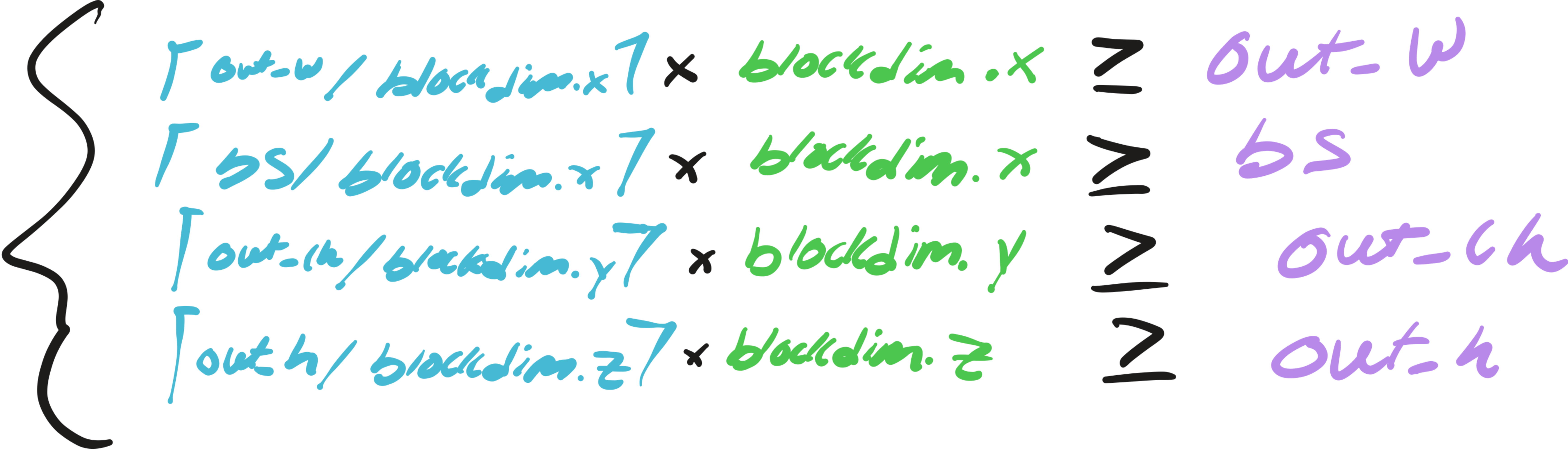
Step 3: Simplify to Total FLOPs:
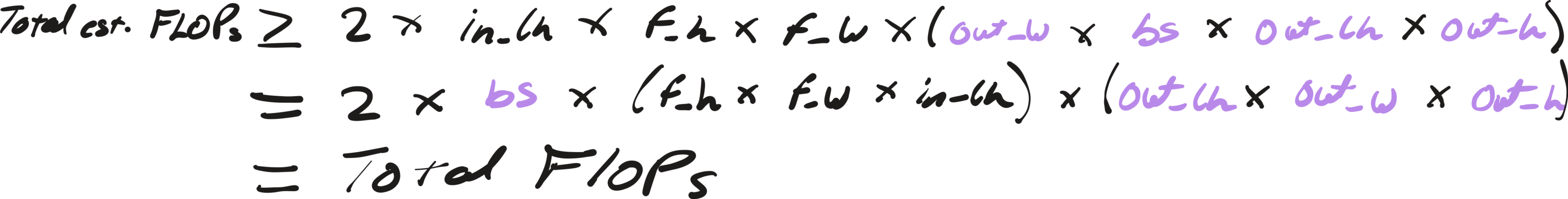
Therefore, Total FLOPs ≤ Total est. FLOPs, with equality when all dimensions divide evenly ("nice").
7.2 Appendix II
The following shows how batch normalization can be embedded into the weights and biases of a convolution kernel post-training:
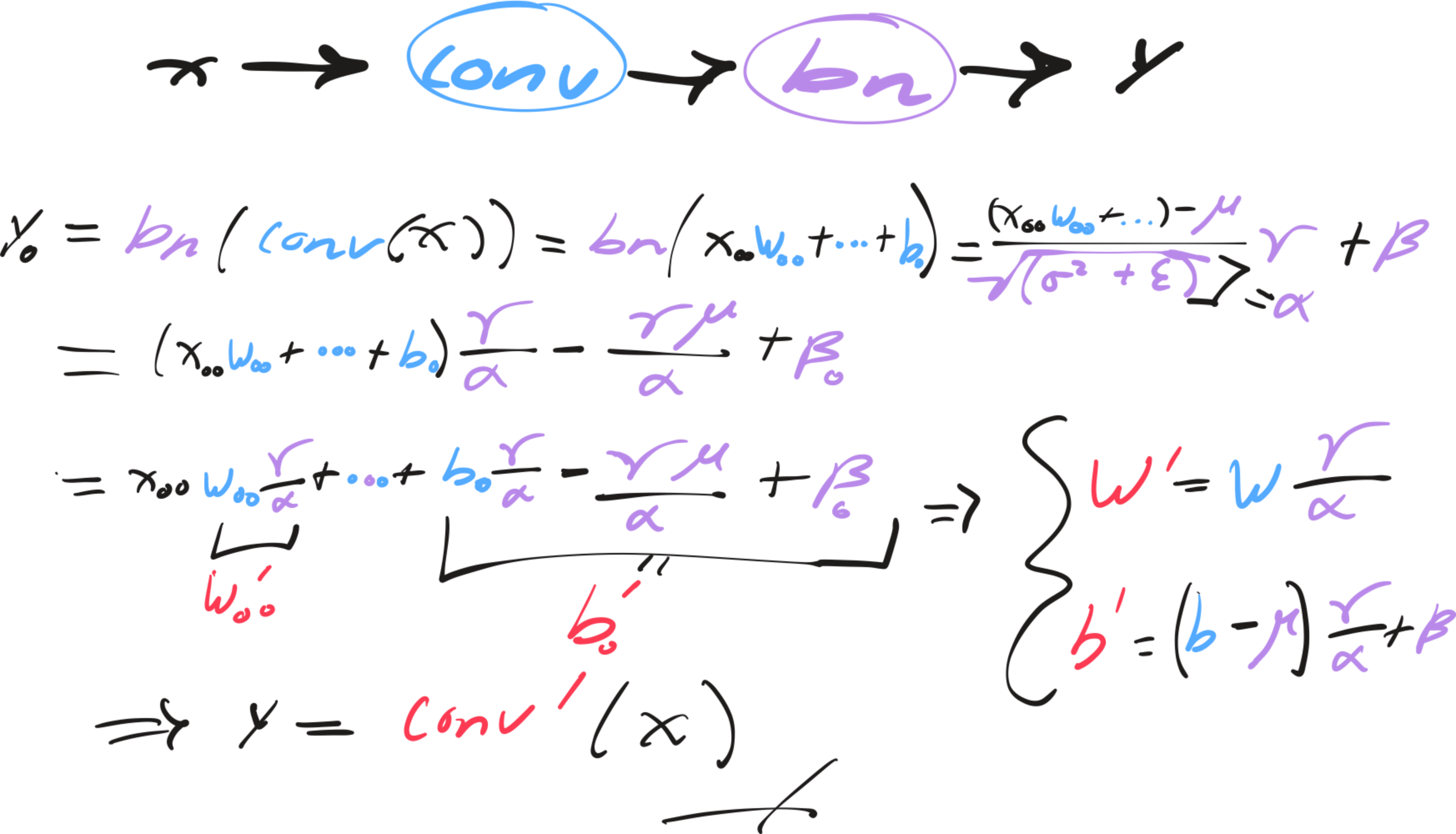
Fig. 17: Derivation for conv-bn folding